How To Use OpenSCAD
Getting Started
Opening the Software
When the program is first launched, we can either make a new file or open an existing one. There are also examples of models and functions provided by the program.
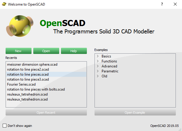
If we choose a new project, we get a screen that looks like this:
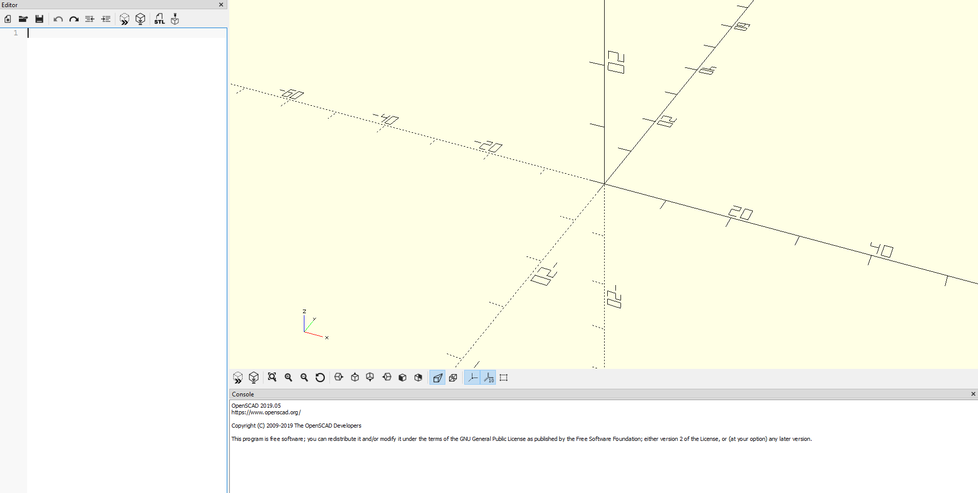
The coordinate system has values but no units, in reality these units are mm. It’s very easy to change the overall size of a model (either in OpenSCAD or later on before printing) so it’s not too important to worry over whether the object is too large/small.
Once this canvas is open, there is 3 main areas of interest. On the left, there is the editor where you can write the code to create the models. The grid is the workspace which will show what you have built so far, and the console will display details of the build when it is created and display any potential error messages.
Cheat Sheet
Open the cheat sheet by clicking help (on menu bar in the top left of the screen), then cheat sheet. This should open a webpage displaying the following:
It outlines what three dimensional shapes can be created along with the format of the code to be inputted. It is also worth noting that the code for transformations that can be applied to objects created is available here.
Noteworthy Points
Commenting
To add comments to your script, type in two slashes followed by the comment you wish to insert. For example, //Comment here.
To comment out several lines of script, type in /* before the section you wish to comment out and then */ after the section.
Language & Syntax
When inputting vectors directly (such as when describing transformations or coordinates) square brackets MUST be used. For example, translate([1,2,3]) represents a translation by the vector [1,2,3] in xyz cartesian coordinates.
Explanation for syntax and notation can be found online at the OpenSCAD User Manual.
Size of Text on Screen
To increase the font size of code press Ctrl and + on the keyboard (or go through Edit, Increase Font Size). To decrease the font size press Ctrl and - (or Edit, Decrease Font Size).
Online Resources
Open Home
Openhome takes you to a series of models that other OpenSCAD users have made and then uploaded to Open Home. Below are some of the more interesting mathematical resources available on the website.
Using Function Grapher
This Openhome Function Grapher is used as a template, we can take this across to OpenSCAD by copy and pasting the code provided on the site. It is worth noting, however, that the first section of code isn’t the best way to create a surface. Scrolling down the page it goes into depth about how the code is produced. To get the best end results scroll to the end of the page and use the last piece of code.
Then change the function to the one you wish to output, as well as making any alternations to the minimum and maximum values. Resolution and thickness can also be changed before printing.
TIP: Mathematical functions available in OpenSCAD (along the code for them) can be found by clicking on the links found on the cheat sheet in the lower rightmost column.
Basic Shapes
Creating Cubes
To create a 3D object in OpenSCAD, type in the code from the cheat sheet into the window at the left-hand side of the screen and then press F5 on the keyboard to preview the object. Later we will press F6 to render the final object.
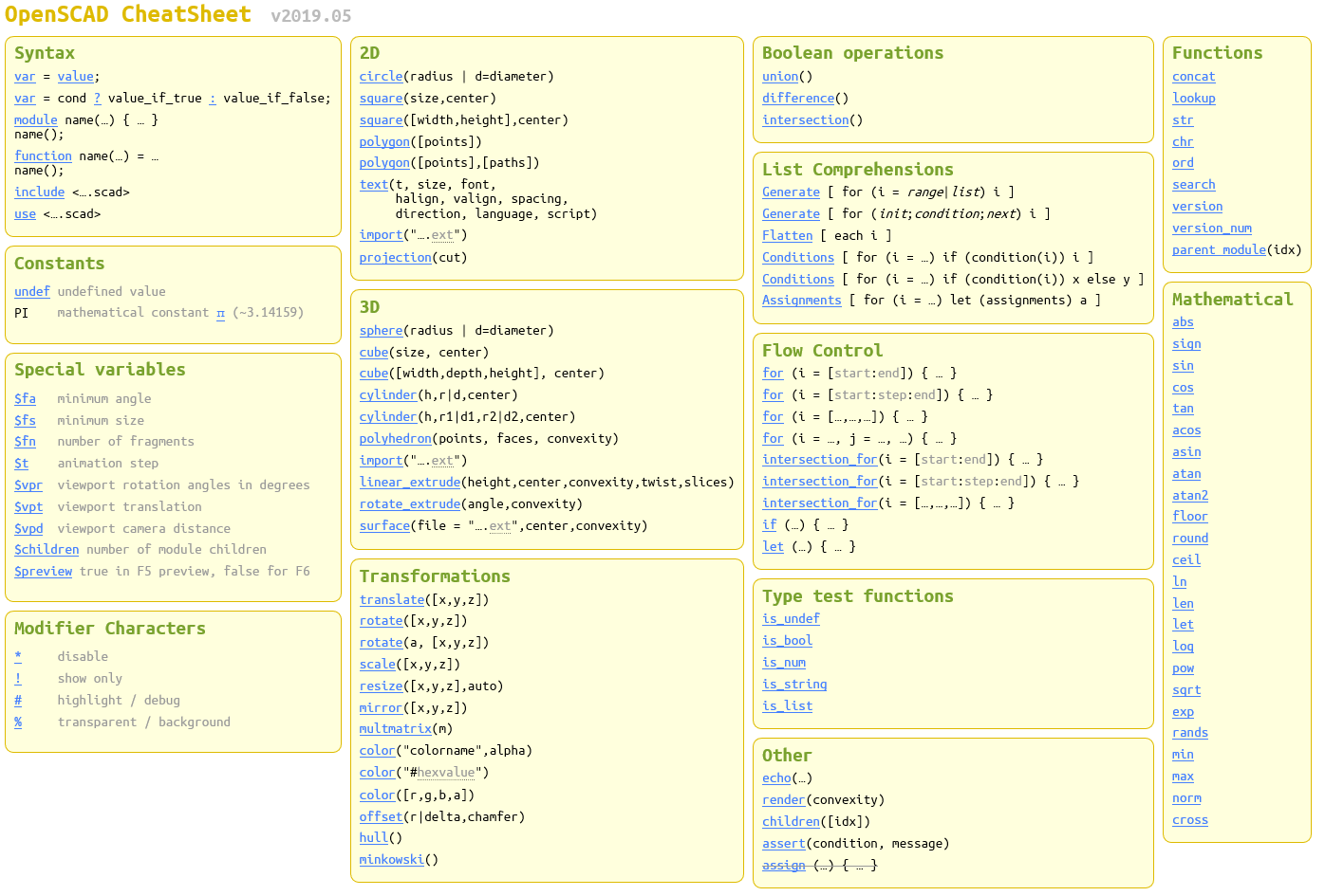
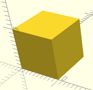
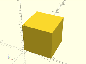
cube(10);
For example, here we have a uniform cube with each side measuring 10mm. As you can see, it places the cube with one vertex at the origin then constructs the rest of the cube in the positive direction.
TIP: Don’t forget to add a semicolon to the end of an object or else you’ll receive a pop-up error.
Centring Objects
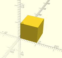
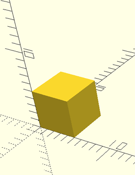
To make the cube centred around the origin, change the code from above to cube(10, true); and this will set centring to true. All objects in the cheat sheet which have the word "center" at the end of the code can be centred in this way.
cube(10,center=true);
This can make transformations easier as the cube is aligned with the coordinate system with which it is being manipulated around.
Creating Cones
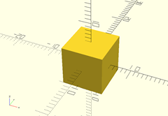
We can create a cone by using the cylinder code and setting one of the radii to be 0. Say we want the cylinder to have a height of 30mm, the base to have a radius of 7mm but we don’t want it to be centred.
cube(10,center=true);
cylinder(h=30,r1=7,r2=0);
As we can see, the cone is built centred around the origin in the x and y plane (due to there being a radius involved and not a vertex) but not along the z axis. Moreover, the cone is placed inside the cube (to change this, see the transformations section). The printer will not recognise these as two different shapes to print separately but print this whole object as one 3D shape.
Creating Circles
To create a 2D object in OpenSCAD, type in the code from the cheat sheet into the window at the left-hand side of the screen and then press F5 on the keyboard to preview the object.
circle(r=4);
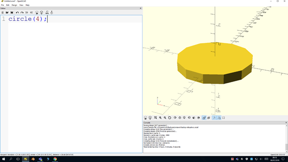
As you can see from the screenshot above, a cylinder with radius 4 has been drawn on the screen when we press F5. However, if you press F6 to try and render it, a red outline filled in green will appear. This is because it is a 2D shape so has no depth and thus there’s nothing to print.
circle(r=4);
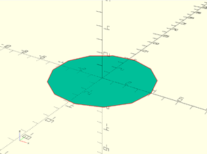
If we want to turn this into something we can print, we can extrude this shape either linearly or rotationally. It is also worth noting that this circle doesn’t have a very smooth edge as you can see the straight edges – to fix this look at the Fragment Number section.
Special Variables
The $fa, $fs and $fn special variables control the number of facets used to generate an arc. From the screenshots of the circle, you may notice that the circle is made up from several straight lines. To make the arc smoother and look more like a circle we can change the special variables $fa and $fs or just $fn. Changing the fragment number (fn) is the easiest way to produce a smooth arc or surface.
However, it is also possible to do by changing the minimal angle ($fa) and size of fragment ($fs) at the same time (if you only alter one, the other will just remain at its default value). When this method is used, OpenSCAD will use a minimum of 5 fragments when rendering a circle and usually one of the variables will limit the other.
Fragment Number $fn
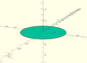
By using $fn= we can increase the number of fragments and increase the smoothness; by default, it is set to 0. Setting this value to be greater than 0 results in both the $fa= and $fs= commands being ignored. It also renders a full circle with the number of fragments set by the value. We could increase the number of fragments to, say, 50 and produce the circle below. The larger the value, the more fragments used (in this case more lines to create the circle arc) so the smoother the edge/surface.
circle(r=4, $fn=50);
TIP: It is not recommended to exceed 100. Below 50 is advisable for performance. This is because the higher number of fragments will consume more CPU and memory. TIP: Keep this value low until the design is complete then change it before rendering to maintain a higher performance whilst building the model.
Alternatively, you can set the number of facets at the top of the code then have it follow through into each shape.
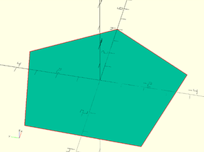
In conjunction with a circle/cylinder, the fragment number can be used create regular polygons. For example, if we were to set $fn=3 OpenSCAD would produce an equilateral triangle and $fn=5 would produce a regular pentagon. The radius of the circle becomes the distance from the centre to each vertex (otherwise known as the circumradius).
circle(r=4, $fn=5);
Minimum Angle of Fragment fa
Decreasing the minimum angle will increase the smoothness.
The default of this is 12, so (360/12 = 30 fragments for a full circle). If this value is changed to a non-integer, it will round up the number of fragments. For example, if we kept the minimum size of fragments at the default then changed the minimum angle of fragment to 70 ($fa=70) OpenSCAD would produce 6 fragments. This is despite 360/70=5.14, which we’d normally expect to round down to 5 fragments. In fact, OpenSCAD will produce 6 fragments up until $fa=71.99995, where any number larger than this would produce 5 fragments.
Minimum Size of Fragment
The default of this is 2, which can be decreased to produce a smoother curve.
TIP: Small circles tend to have less fragments because of this default value, so sometimes it is worth changing this as opposed the fragment number.
Stepping Up
Linear Extrusion
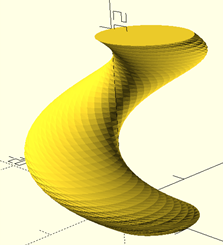
Linear extrusion is a useful tool for making two dimensional objects into three dimensional prisms with that object as a ‘top’ and ‘bottom’ face. Here, we can specify the ‘height’ of the object to create a simple prism and choose whether to have the object centred around the axis or not. We can then also choose if the shape has a ‘twist’ (centred around the z axis) and if so, how many degrees this twist will go through. ’Slices’ can then be used to change the number of horizontal slices the object is made from which in turn makes the shape smoother as it twists upwards.
linear_extrude(height=20,
center=false,convexity=10,
twist=360, slices=40)
translate([5,0,0])
circle(5, $fn=40);
Rotational Extrusion
The other method for creating a three-dimensional object from a two-dimensional shape is using rotational extrusion. We can create an initial shape, and when we rotationally extrude it, it is assumed to be in the x-z plane. Then, we can specify the angle the shape can be extruded through, again around the z axis.
rotate_extrude(angle=90)
translate([10,0,0])
circle(5, $fn=40);
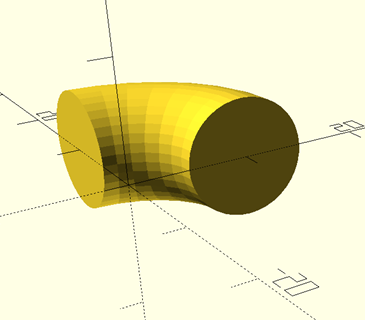
TIP: Linear extrusion will occur in the positive z direction and rotational extrusion will occur anti-clockwise around the z axis. TIP: For rotational extrusion, the shape must be fully in the positive x direction. Therefore, a translation or rotation may be required to position the shape in this region.
Command |
Action |
|
Creates a square or oblong with specific dimensions,and a centre point. |
|
Creates a multi-sided shape around specific, oriented points that are specified in the array. |
|
A prism-based extension of the circle. The latter command creates a cylinder with varying width at the start and end faces. |
Transformations
Translation
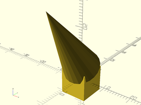
If we want the cone to be placed on top of the cube, we’d need to apply a transformation to it. In this case a translation by 5 units in the z direction would work since the cube’s surface is 5units above the origin where the cone’s base is. To do this, type the transformation in the line above the object you wish to apply it to. The object that it is applied to is called the child.
cube(10, center=true);
translate([0,0,5])
cylinder(h=30,r1=7,r2=0);
Since we are dealing with coordinates now, we must type this in square brackets to make a vector.
TIP: You don’t need to add a semicolon to the end of this line as it is a transformation which applies to the next line.
To perform a single transformation on multiple objects, add curly braces around the objects the transformation will apply to rotate()
Multiple Transformations
We can also do multiple transformations consecutively.
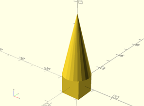
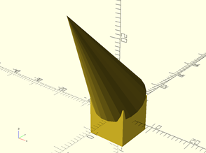
For example, say we wish to translate it up 5 units and then rotate the cone around the x axis by 35. We’d write out the code for the rotation in one line, then the code for translation in the next line and finally the code for the object in the last line.
cube(10, center=true);
    rotate([35,0,0])
    translate([0,0,5])
    cylinder(h=30,r1=7,r2=0);
Order of Transformations
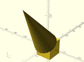
The order of transformations is very important; if we wanted to do the rotation then translation we’d end up with a different object as shown below:
cube(10, center=true);
    translate([0,0,5])
    rotate([35,0,0])
    cylinder(h=30,r1=7,r2=0);
This screenshot is taken from the same camera angle and position, so the differences are quite apparent – in this case the cone has merged into the cube.
TIP: Take care with the order transformations are coded. Transformations are applied from the bottom up.
rotate([35,0,0]) translate([0,0,5]) shape;
Takes the shape and then applies the translation to it. Then this takes the result of that and applies the rotation to it.
Boolean Operations
Union
Suppose we wish to treat the cone and cube as a single object. We can create a union. The cheat sheet only mentions union() but to select the objects (can be more than 2) for this to be performed on curly braces are used.
union() {
    cube(10, center=true);
        translate([0,0,5])
        rotate([35,0,0])
        cylinder(h=30,r1=7,
        r2=0);
}
It is worth noting that transformations to individual objects can be applied within the union (e.g. the ones applied to the cone remain despite it being part of the union).
In terms of Boolean operators, this is the equivalent of OR.
Difference
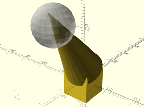
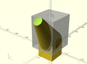
We can use difference to cut an object. If we want to cut out an object into it we use a similar method to union – we type out difference() and then curly braces around the object we wish to cut out of as well as the shapes we wish to cut. The first object to be coded in the curly braces is the one which shall be cut into. All subsequently coded objects in the curly braces are the shapes that will be removed from the initial object.
The easiest way to think about it is if we were to place a sphere with radius of 6.5mm on the end of the unified shape and then remove all the object which was contained within the sphere. In this case the unified object would be the initial object (and thus MUST be coded FIRST) and the sphere is the subsequent object which will be cut into the initial (and is thus coded on the lines AFTER the initial object). The easiest way to think about it is if we were to place a sphere with radius of 6.5mm on the end of the unified shape and then remove all the object which was contained within the sphere. In this case the unified object would be the initial object (and thus MUST be coded FIRST) and the sphere is the subsequent object which will be cut into the initial (and is thus coded on the lines AFTER the initial object). It is worth noting that transformations and various operations can all be applied within the difference (e.g. union, translation and rotation occur in this case).
difference() {
    union() {
        cube(10, center=true);
            translate([0,0,5])
            rotate([35,0,0])
            cylinder(h=30,
            r1=7,r2=0);
    }
    translate([0,-15,25])
    %sphere(6.5);
}
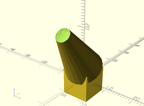
TIP: Placing a percentage sign % before an object will make it transparent, in this case we can still see the end of the cone. Placing an octothorpe # before an object will highlight the object in red and perform the operations on it.
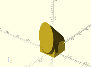
After removing the % from the line of code with the sphere on we can see what the difference operation does.
difference() {
    union() {
        cube(10, center=true);
            translate([0,0,5])
            rotate([35,0,0])
            cylinder(h=30,
            r1=7,r2=0);
    }
    translate([0,-15,25])
    sphere(6.5);
}
In Boolean operators, this is the same as the first object coded NOT any subsequent objects coded.
Intersection
We can produce an object which is the intersection of multiple objects. To do this, use the intersection() command in the same way as the we would use union.
For example, if we want to take the intersection between the previous object and a cuboid which is shown in the grey below:
intersection() {
    translate([-9,-6,0])
    %cube([15,16,20]);
    difference() {
    union() {
        cube(10,
        center=true);
            translate([0,0,5])
            rotate([35,0,0])
            cylinder(h=30,
            r1=7,r2=0);
        }
        translate([0,-15,25])
        sphere(6.5);
    }
}
We would get this:
intersection() {
    translate([-9,-6,0])
    cube([15,16,20]);
    difference() {
    union() {
        cube(10,
        center=true);
            translate([0,0,5])
            rotate([35,0,0])
            cylinder(h=30,
            r1=7,r2=0);
        }
        translate([0,-15,25])
        sphere(6.5);
    }
}
This is the same as the Boolean operation AND it is the result of taking all the parts that are present in both shapes.
Introducing Variables
An important aspect to coding is making the code easy to follow and edit. To achieve this, it is often best to turn certain values into parameters which can be edited without having to trawl through code and prevents the need to make repeated changes.
It is straight forward to do, state the parameter and make it equal to a value followed by a semicolon. The code length = 10; would set up a new variable up called length and set its value to 10.
length = 10;
cube(length);
Now we can change the length of the cube with ease. Say we wish to change the uniform cube to be 5mm long:
length = 5;
cube(length);
Everywhere the variable appears in the code can now be changed in one place and in one go, rather than repeatedly throughout the code. It also reduces the risk of looking through the code to find which parts need altering and potentially missing some of the times it appears (especially in long or complicated code).
Text
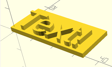
Another good feature of OpenSCAD is the ease with which text can be used on other shapes. Simply by using the text("...") command, any text can be created and used. The size, font, and many other features of this can be changed, and a simple translation and difference command allows text to be cut out of other shapes.
translate([-1,-1,0])
    cube([35,16,2]);

linear_extrude(height=4)
    text("Text!", size=11);
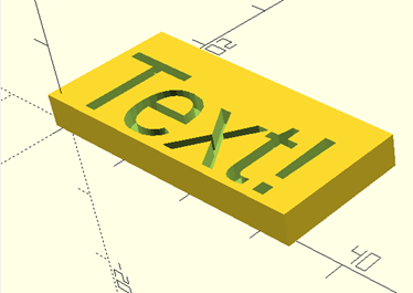
Now, we can use the Boolean operation difference(); with the text to create a shape with text indentation:
difference() {
    translate([-1,-1,0])
        cube([35,16,2]);

    translate([0,0,2])
    linear_extrude(height=4)
        text("Text!", size=11);
}
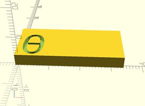
Special characters are produced by writing their Unicode code after a backslash. For example, if we want to engrave into a block, we would change the "Text!" to be \backslash u03B8 as this is the source code for .
difference() {
    translate([-1,-1,0])
        cube([35,16,2]);
    translate([0,0,2])
    linear_extrude(height=4)
        text("$\backslash u03B8$",size=11);
}
Interlocking Pieces
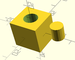
For some models, there will need to be multiple pieces that fit together and move. Therefore, having a peg and a hole for example could be useful. Due to the resolution and accuracy of the printer, it is important to allow margin for error to ensure pieces will fit together. It is probably best to allow 0.5-1.0mm difference in diameter between pieces; for example a 9mm diameter peg and a 10mm hole.
difference() {
    cube(20, center=true);
    cylinder(h=10,d=10,$fn=20);
}

translate([20,0,0])
    cylinder(h=10,d=9,$fn=20);
Importing Files
OpenSCAD can import files containing models for you to edit. This is can be done by using the import function – using code of the format import("PATH LOCATION/NAME.FILETYPE");. Notice how there are quote marks in the code around the file name.
import("filename");
To find the file path, right click the file and go into properties.
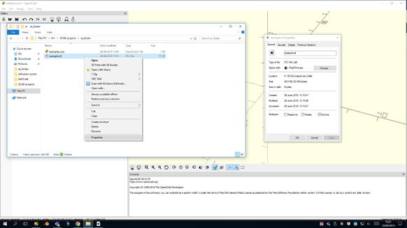
Copy and paste the location into the speech marks. ON WINDOWS YOU MUST CHANGE THE BACKSLASHES TO FORWARD SLASHES!
import("H:/SCAD projects/ex_folder");
Then type another forward slash followed by the file name and then the file type, in this case .stl.
import("H:/SCAD projects/ex_folder/example.stl");
Press F5 to preview and F6 to render. Then you can treat the import as a single object and apply other transformations to it as you would normally.
TIP: The easiest way to import a file is by draggin the file into the command window (where code is typed in) and copying it across. TIP: You can also import .dat files, which is rather useful in conjunction with the surface(); function.
Surface Function
Data to OpenSCAD
The surface(); function creates an surface by reading heightmap information from text or images. In text-based files, OpenScad requires an input of a matrix of z coordinates, where the rows are mapped to the y axis and the columns are mapped to the x axis. It follows that the first column will be plotted along the x axis and thus have x coordinate 0, then the second column will be plotted along the line x=1.
For example, if we use notepad to type out:
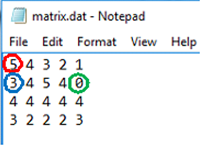
Then this would plot a surface which includes the coordinates at [0,0,5], [1,0,3], [4,1,0] (shown with the same colour coordination further down).
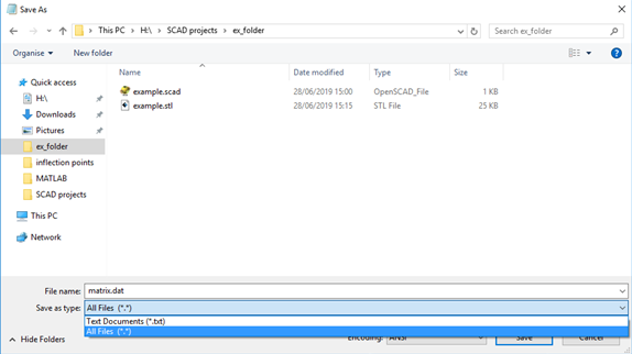
Then save this as a .dat file by clicking: File, Save As, then the drop down and selecting All Files (*.*). In the File name type out the name you wish to save it as then .dat (as shown below).
To turn the .dat file into a surface, use the same method as importing an .stl file with two slight changes. First is to replace the word import with surface (to form the surface). The second is to replace the .stl with .dat after the file name (to read the file correctly).
import("H:/SCAD projects/ex_folder/matrix.dat");
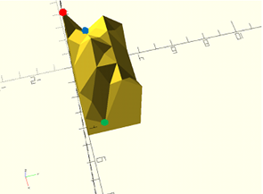
As you can see, this function provides a base below the model to allow for solid printing. If you wish to reduce the size of this base, use the difference() function with this surface and subtract a translated cube (with an equally sized or larger area than the base) to remove the lower section.
MATLAB to OpenSCAD
An alternative to using the function grapher is to plot a surface using MATLAB then import it into OpenSCAD. The method for this can be found in a separate guide called ‘MATLAB’.
More Advanced Tools
For Loops
It is simple enough to create 2 cubes and then translate one of them so there is a gap between. However, if we wish to move 50 cubes to each have an equal gap between them it would be a rather long process to do manually. To reduce the amount of work required, a for loop can be introduced to produce the same result.
To make things simpler, this code will include variables (see the ‘Introducing Variables’ section above for further information on this).
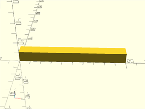
To begin with, suppose we have a uniform cube with each edge 10mm long.
length=10;
cube(length);
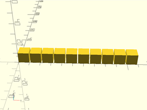
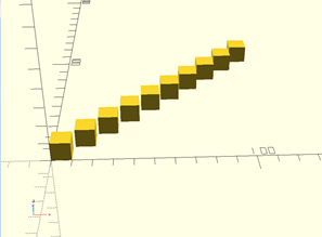
Next, we’ll introduce a for loop to generate 10 cubes positioned next to each other, starting from the origin and ending at 100mm.
length=10;
for (i = [0:9]) {
    translate([length*i,0,0])
        cube(length);
}
TIP: In the code we’ve used 10 iterations from 0 to 9, rather than from 1 to 10. If we’d started from i=1 then the first cube would’ve been translated by [1,0,0] and ended up away from the origin then every other cube would also be shifted along one in the x direction. If we wanted to, we could use iterations from 1 to 10 then translated by [length*i-1,0,0].
Now suppose we want to have a gap between each of the cubes, say, of size 1mm.
length=10;
gap=1;
for (i = [0:9]) {
    translate([(length+gap)*i,0,0])
        cube(length);
}
TIP: Here we’ve included the gap in the brackets with the length, else it would’ve just translated the whole block along by 1mm instead of each individual block by an extra 1mm.
If we want to produce a 10 by 5 grid of the cubes with a gap of 1mm on round every edge, we’ll need a nested loop function.
length=10;
gap=1;
for(j = [1:4]) {
    for (i = [0:9]) {
        translate([(length+gap)*i,(length+gap)*j,0])
            cube(length);
    }
}
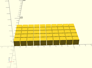
This is because we have the 10 i iterations to go through PER EACH j iteration. Since we have 5 iterations of j and 5*10=50, we have 50 iterations in total and thus 50 cubes. In other words, the j=0 iteration is producing the first row of cubes at y = 0, the j=1 iteration is producing the next row of 10 cubes along the line y=11 (10 for length + 1 for gap) and so on.
If we didn’t have a nested for loop the first issue would be the number of iterations being different in i and j. The other issue (more importantly) would be that the total number of iterations would be wrong. As there would still only be the 10 i iterations, rather than the 50. To illustrate this, if we left it as a single for loop (and change the j to an i since there is no longer a for loop with a j) we’d have a single set of 10 cubes spaced along the line y=x.
length=10;
gap=1;
for (i = [0:9]) {
    translate([(length+gap)*i,(length+gap)*i,0])
        cube(length);
}
Modules
When it comes to combining shapes, it is useful to group transformations and unions etc together to save repletion of long lines of code, which is where modules come in. These act in a similar way to functions in languages like R, in the form module ModuleName() {...}.
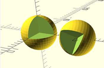
Now, we can recall a specific module and transform it so all parts of the module will undergo the same transformation, and even use functions to combine or find the difference between two modules.
module MyShape() {
    difference() {
        sphere(4, $fn=40);
        cube(4);
    }
}

MyShape();

translate([0,10,0])
rotate([45,45,0])
    MyShape();
Functions
Functions work in a similar way: inputting a certain variable or value will produce another value. Functions can then be used inside modules or loops to give the output when certain input values are put into the function. This function takes an input value of and produces the value of as the output, which is represented by the z coordinate of each cube.
function quad(x) = pow(x,2) - 2*x + 1;

module plot() {
    for (i = [-5:5]){
        translate([2*i,0,0])
            cube([1,1,quad(i)]);
    }
}

plot();
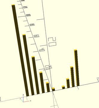
The key difference between modules and functions is that modules work with shapes whereas functions produce values such as numbers and vectors. For example, we could have written the function specified in the example above in the coordinate part of the cube dimensions, but specifying a function beforehand means larger, more complicated code can be simplified.
Saving and Exporting Files
Saving Files
You can save your OpenSCAD script as a .scad file so you can save and edit it later by going through File then Save as. Then save the file as you would any other, by typing the file name.
TIP: It is often better to name files without spaces between words; a solution is typing – or _ between them. For example, ‘example number one.scad’ would be better written as ‘example-number-one.scad’ or ‘example-number_one.scad’.
Exporting Files
To take the final model and export it as a readable file, it needs to be rendered first. This is done by pressing F6 on the keyboard. Typically, this will take longer than previewing (pressing F5).
After the model has rendered, select file, export and then chose which file is most suitable (in most cases .stl). The shortcut for exporting as an .stl is F7. For the file to properly export and save as an .stl file, you must wait for the console to display a message saying ‘STL export finished:’ followed by the path location and file name. Otherwise, there may be errors later during printing.
TIP: If you try exporting without rendering, an error message will appear in the console and it will not export.
Examples
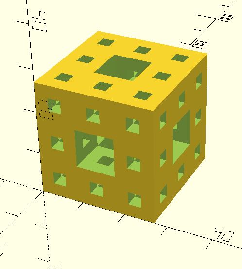
Menger Sponge
The Menger Sponge is a three dimensional fractal, where there is a self similarity to the shape. To create the shape, a cube is split into 27 smaller cubes, and the middle cube from each face is removed as well as the centre cube. This the repeats indefinitely to create a fractal.
Let us try to create a Menger Sponge. We will begin with a base cube and build up rather than removing cubes for this demonstration.
We begin by defining variables. Say ‘unit’ represents the length of the base cube and ‘hole’ represent a third of this, the segment that will be cut out.
unit=9;
hole=unit/3;
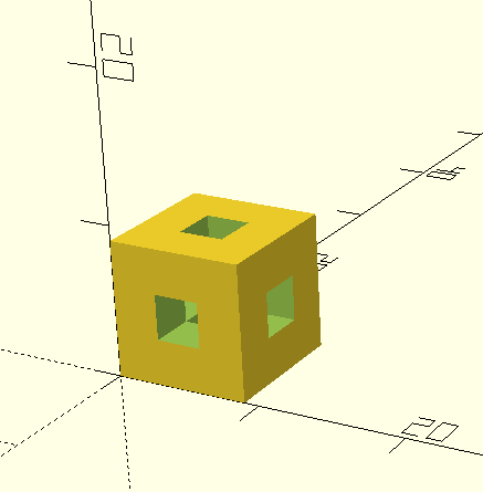
We can then create a module for the first iteration of this model. We have called it ‘cube1’. We then use the difference command to ‘cut out’ three 9x3x3 blocks from the base cube. This will mean all the required cubes are removed in 3 commands.We then call cube1 to reveal what we have so far.
module cube1() {
    difference() {
        cube(unit);
            translate([0,hole,hole])
            cube([unit,hole,hole]);
            translate([hole,0,hole])
            cube([hole,unit,hole]);
            translate([hole,hole,0])
            cube([hole,hole,unit]);
    }
}

cube1();
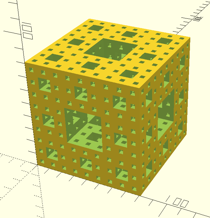
Now we begin the iteration. A for loop is good practice to use in these situations to save writing similar lines lots of times. The first triple nested loop will create a larger cube which is 3x3x3 of the base cube. Again we have used a difference command, so now we remove the same blocks from the cube, which are now 27x9x9 as we have scaled up. The first for loop means we translate to a specific x and y coordinate, and travel in the z direction removing the cubes we reach there. The following loops do the same in the x and y directions. We then call ‘scaledcube1’ to see where we are
module scaledcube1() {
    difference() {
    for (i=[0:2])
        for (j=[0:2])
            for (k=[0:2])
                translate([i*unit,j*unit,k*unit])
                cube1();
        for (i=[0:2])
            translate([unit,unit,i*unit])
            cube1();
        for (i=[0:2])
            translate([i*unit,unit,unit])
            cube1();
        for (i=[0:2])
            translate([unit,i*unit,unit])
            cube1();
    }
}

scaledcube1();
Now we know this module works, it is simple to scale up another iteration. We define ‘unit2’ to be three times greater than ‘unit’, and then replace all ‘unit’ in the previous module with ‘unit2’, and name the new module ‘scaledcube2’. When we call this, we see another iteration has occurred. Therefore defining unit3, unit4 etc and repeating will give us a larger and larger Menger Sponge with more intricacies.
unit2=3*unit;

module scaledcube2() {
    difference() {
    for (i=[0:2])
        for (j=[0:2])
            for (k=[0:2])
                translate([i*unit2,j*unit2,k*unit2])
                scaledcube1();
        for (i=[0:2])
            translate([unit2,unit2,i*unit2])
            scaledcube1();
        for (i=[0:2])
            translate([i*unit2,unit2,unit2])
            scaledcube1();
        for (i=[0:2])
            translate([unit2,i*unit2,unit2])
            scaledcube1();
    }
}

scaledcube2();
TIP: It is good practice to use as few variables as possible and have as many other variables in terms of these starting few. This means less needs to be changed if the model needs scaling for example.
Troubleshooting
Issue |
Cause of Issue |
Solution |
Models not rendering |
Specific shapes and modules may not have been recalled correctly |
Call all shapes you require and make sure all shapes are closed with a semi-colon. Also, double check spellings as OpenSCAD uses American English (center rather than centre) |
Shapes not appearing |
In an F6 render, the shapes recalled may not appear due to being two dimensional |
Linearly extrude the shapes so they become three dimensional prisms that are able to be rendered. |