We fixed the longest and shortest wavelengths to be 1 (i.e the box size) and 0.123091487 respectively.
This meant that the Reynolds number was approximately 16.3 throughout.
We used 5 values for eta, ranging from 5e-4 to 2e-2. The following graph shows the evolution of magnetic field strength for each simulation.
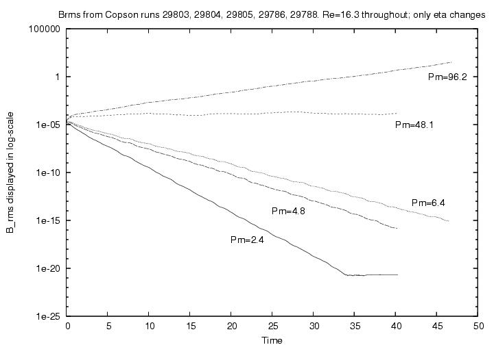
As we can see, when the magnetic Prandtl number increases, we move from a regime in which the magnetic energy decays
to one where the magnetic field strength grows - i.e. we have dynamo action!
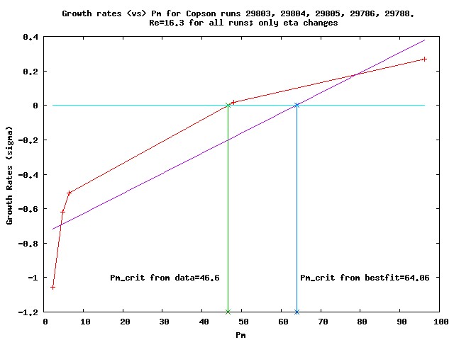
We have measured the growth rates, (sigma) for each of the simulations above. This is plotted as a function of Pm in the figure below.
From the data, we can see that the critical value for Pm at which dynamo action is initiated is somewhere between Pm=46.6 and Pm=64.04.
It may also be interesting to see how the magnetic field looks:
are there any notable differences between the isosurfaces of a decaying magnetic field and those of a growing field?
The figures below suggest a marked difference; the first 3 pictures show a time evolution of the magnetic field strength (displayed as isosurfaces with the level set at 2*Brms in each case) for a run in which there was no growth of magnetic energy. The second set of 3 pictures show a dynamo run at the same instances in time. As we can see, the dynamo has many more small scale features and it exhibits elongated structures - evidence that the turbulent flow field is stretching the magnetic field.